Here are two commented examples of use of QuickPlotLib to illustrate our introduction: a basic first one, then a more sophisticated example.

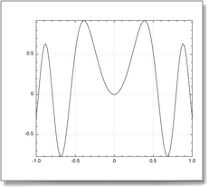
Plotting a function y = f(x) with QuickCurve

QuickCurve({-1, 1}, "cos(x)*sin(10*x^2)", 0)

Import script

The prototype for QuickCurve is QuickCurve(x, y, object). To plot a function, we pass the range {-1, 1} for x and the formula "cos(x)*sin(10*x^2)" for y. Specifying 0 for the object is what you do by default: the new curve will come in a new window.

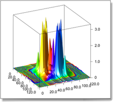
Viewing the spectrum of 2d field with QuickFFTSurface

Viewing the spectrum makes more often sense for data which come from experiments. Here we do not have an experiment, so we shall plot the spectrum of an analytic function.

set nc to 128
set nr to 128
set x to creatematrix "x" ncols nc nrows nr range {0, 2 * pi} as matrix
set y to creatematrix "y" ncols nc nrows nr range {0, 2 * pi} as matrix
set {x, y, z} to QuickFormulaMatrix(x, y, "sin(2*(x^2+y^2))*sin(2*sqrt(x+y))")

QuickFFTSurface(z, "FFT")

Import script

creatematrix is discussed in the Chapter about the Scientific environment. creatematrix makes a 2d matrix with the specified sizes. The "x" or "y" parameter is how you initialize it with x or y values.
QuickFormulaMatrix(x, y, formula) returns the matrix obtained by evaluating the formula for the values of x and y provided in the x and y parameters.

Finally, QuickFFTSurface(z, object) computes the 2d Fast Fourier transform of its z argument. QuickFFTSurface plots the modulus of the Fourier transform as a surface f(x,y). The phase of the Fourier transform is mapped into the color of the surface: the color scale is [-pi, pi].

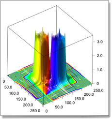
The other example was obtained using a different formula.